Getting Started with Geospatial Functions

Geospatial data is any data that has a geographic component to it. A geographic component simply implies a location (or a set of locations) that can take the form of simple points on a map with latitude and longitude coordinates or more complex shapes that describe lines and boundaries, or even elevation. Examples could include a country’s border, a line representing a road or a river, or the outline of a lake. 

Geospatial data often combines geographic information about a location with other associated attributes. For instance, line geometry describing a road could be combined with information on traffic, or shape geometry that describes a county could be combined with poverty rates, vaccination levels etc.

Geospatial data is commonly housed in a geographic information system (GIS). Popular examples include ArcGIS, PostGIS, QGIS etc. Kinetica takes GIS a step further for analysis of larger volumes of streaming geospatial data – such as you might find with IoT and moving devices. Kinetica provides over 130 geospatial functions modeled on the Spatial Type (ST) spec developed by the OpenGIS Consortium (OGC). These geospatial capabilities are made available on top of a highly performant, vectorized data platform, but the ST functions remain similarly intuitive.

However, the vast array of functions can be intimidating, especially if you are unfamiliar with geospatial analysis. This post provides a framework to help you classify and think about geospatial functions which will make it easier to become productive quickly with geospatial data and analysis. 

We will start by classifying the functions by the type of spatial operations they perform.

Types of functions

These functions can be broadly classified into three groups based on the type of things that we can do with them.

The first group are functions that compute spatial attributes. Attributes describe particular aspects of a geometry such as the area and perimeter of a polygon, the length of a linestring, the min and max values for a geometry etc. 

The next set of functions describe the spatial relationships between different geometries. These help us answer questions such as:

• Do two geometries intersect? 
• Are a set of points contained by another polygon? 
• What is the distance between two geometries?
•  Are two geometries equal? 
• Where is a particular geometry in reference to another?

The third set of functions construct new geometries either from scratch or using other geometries. Some examples of these include: 

• Constructing the centroid of a polygon
• Drawing a buffer around a particular geometry
• Creating new shapes through the intersection or the union of shapes
•  Spatially aggregating existing geometries into a larger geometry

When combined, these three broad categories of functions can be used to cover a wide range of geospatial analytics use cases. Let’s explore those:

Analytical Use cases

Filtering data

The first one we will look at is filtering data. Filtering is a very common analytical operation that is used to identify records in a table that meet a particular criteria. 

In the case of geospatial data, these criteria can be a spatial attribute or a spatial relationship. 

Let’s first look at an example that uses a spatial attribute. Say we have a dataset with all the states in a particular country. We would like to filter and keep all those states that have an area greater than a particular threshold. We can use the spatial attribute function ST_AREA to compute this area and then use that to identify all the states in the data that have an area greater than that value.

Now let’s look at a case that uses a spatial relationship. Let’s say we have a database with the cell phone locations and we want to identify all the phones that are say 1000 meters from a particular cell tower. We can do that using the ST_DWITHIN function, where D stands for distance to filter all the cell phones that are within 1000 metres from the tower.

Joining data

Next let’s check out spatial joins. Joins  involve combining two different tables based on some criteria. In geospatial analysis this typically involves the use of a spatial relationship between the geometries.  For instance, let’s say that the table to the left has county level geographic boundaries and demographic information for the state of New York in the United States, and the one to the  right has information on the locations and characteristics of all the hospitals in the US. Now say we want to identify access to healthcare resources at the level of counties in New York. We can do that using a spatial join that identifies all the hospitals that are spatially contained within each of the county boundaries. Now we have a single table that contains all the information that we need to understand access to healthcare resources within counties in New York state.

Summarizing data

Summarizing is a way to calculate aggregate statistics about the data. 

This is usually performed by grouping the data along a particular categorical variable before computing a summary attribute within each group. For instance, say we have a table with a geometry collection column that contains the borders of states and the roads in them. 

A plausible analytical task for this type of data could be to calculate the total length of roads for each state in the table. We can do this by grouping the data by the states and computing the total length of the roads within each group using, say, an attribute function like ST_LENGTH.

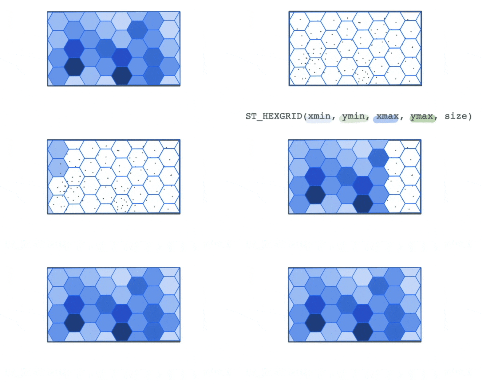
Another aggregation technique that is particularly relevant for the type of large datasets that Kinetica deals with is called binning. Binning involves aggregation of data into spatial buckets so that we can visually see the summary statistics for the data. 

For instance, let’s say we have a large dataset with the location and type of traffic incidents across the US. 

The plot of this data might look something like this. At first glance it is hard to observe any meaningful trends from just looking at the most granular level of data.

However, we could use the bounds of this data to create a new spatial hex grid layer using the ST_HEXGRID function. This grid can then be spatially joined with this data. 

This allows us to  group the traffic incidents based on the bins to calculate summary statistics that can allow us to draw more meaning from the data visually than simply looking at the most granular level of data. 

Bringing it all together

Consider the following challenge. We have two datasets. The first one has information on the location of vehicle breakdowns, with additional information on whether it happened on a highway or not. And the second showing spatial distribution of vehicle owners. 

Now let’s say we are a car servicing company that would like to decide the location of service stations such that they are close to breakdown hotspots on highways and in an area of the town with a high density of vehicle owners. 

Finding vehicle breakdown hotspots can be done by following the steps similar to the one we explored earlier with summarizing the data using the ST_HEXGRID. Once the grid is placed on top of the vehicle breakdown data we can aggregate the breakdowns to find hotspots. We could do something similar to find the areas of town with a high concentration of vehicle owners. 

The next step would be to create a buffer around the vehicle breakdown hotspots and spots with high concentration of vehicle owners. The intersection between these buffers can then give potential spots for where to place a service station.

Summary

Hopefully this gets you started with the basics of using ST Geospatial functions. The next step is to try this out with real data. The Developer Edition of Kinetica is easy to set up, and comes with a variety of datasets and guides that will help you become more familiar with analyzing geospatial data.

For more information on the entire list of geospatial functions available in Kinetica, please visit: https://docs.kinetica.com/7.1/geospatial/geo_functions/

And visit other pages on this site to see how Kinetica makes it possible to do real-time analysis of large volumes of devices moving through time and space,