An Introduction to OLAP for Data Analytics

Data is a critical part of modern businesses. Almost all of our interactions with businesses – online or otherwise- end up touching a business decision system that is based on data. These decisions affect the quality and type of services that are offered to us and have significant implications for the bottom line.

This post introduces some of the key terms and concepts that govern the process of drawing meaning from business data and informing operational and strategic choices. We’ll start by understanding the differences between databases that deal with two types of business data -transactional and analytical. We will follow this with a dip into the world of OLAP data warehouses and then wrap things up with an example.

OLTP vs OLAP

Traditionally, business activities with databases can be classified into two broad categories – Online Transaction Processing (OLTP) and Online Analytical Processing (OLAP).

OLTP systems are designed to accurately capture and validate real time business transactions such as card swipes at a turnstile, movement of inventory, bank transactions, etc. 

Accuracy and speed are crucial for these systems since critical functions, such as a bank balance, need to be reflected immediately and without error for businesses to operate smoothly. 

OLAP systems on the other hand are designed to find meaning from data. Traditional OLAP systems tend to be slower, analyzing historical data in batches collected over a period of time. They are more concerned with the ability to execute complex analytical queries that can deliver business insights than they are with speed.

Let’s use an illustrated example of a person withdrawing money from an ATM to further understand the differences between OLTP and OLAP

A typical OLTP query in this scenario would establish whether this person has enough money in his account to make the withdrawal. An OLAP query, on the other hand, might evaluate whether this person should be sent an email offering a personal loan.

The OLTP query is a simple one and requires the system to check only one thing: the amount of money this particular person has in their account. The OLAP query, however, is far more complicated. The model that determines whether a person should be offered a personal loan could involve the entire history of their account to simulate future cash flows, third party information on credit scores, and demographic information such as their age, income, education, etc. OLTP queries touch just a small portion of the data, such as an account balance, while OLAP queries bring together large portions of the data to provide an answer.

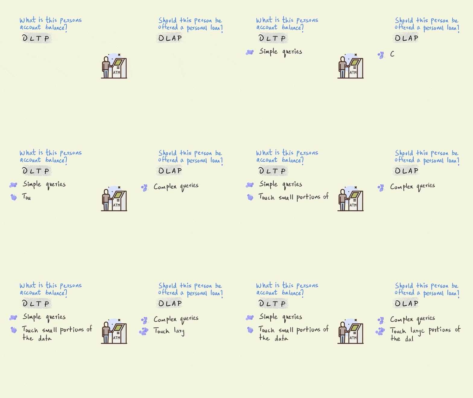
If we zoom out a bit from this single withdrawal, we would also see that there are thousands of such withdrawals happening every minute across all of the bank’s ATMs. So although OLTP queries are relatively simple, their frequency is very high. 

OLAP queries, in contrast, can be executed less frequently. For instance, a company sending email offers on a monthly cadence would need to run the particular OLAP query only once every month.

This illustration presents a stark dichotomy between OLTP and OLAP. 

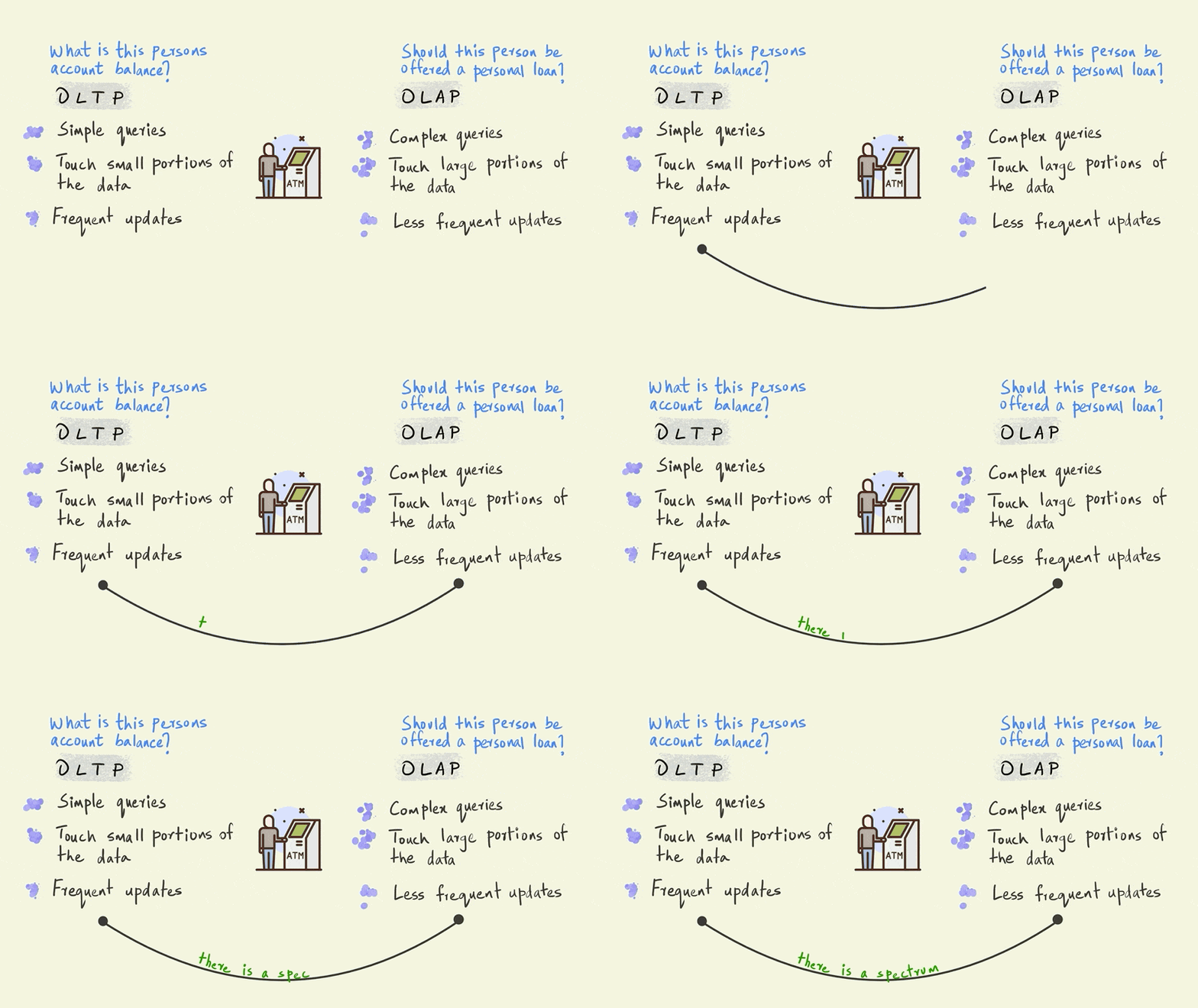
In reality, however, there is a continuum between OLTP and OLAP depending on the type of business use case. 

Moreover, cutting edge solutions like Kinetica are blurring these edges by blowing away some of the previous constraints faced by OLAP systems. Unlike traditional solutions that would only be able to analyze data in batches well after the data is collected, Kinetica is so fast that it can execute these complex queries in real time as the operational data is streaming in. This opens up a whole new suite of business opportunities that were previously impossible. 

For instance, now, we could send a message offering a loan to the person immediately after they perform a withdrawal – striking while the iron is hot – rather than at the end of the week or  month.

Data warehousing

Let’s dive a bit deeper into analytical databases by looking at a related concept – data warehousing. Large businesses typically have multiple OLTP databases that handle different parts of their business operations. Imagine for instance, an online store like Amazon. They would need separate systems to process orders, capture customer behavior on the website, manage deliveries, update inventory, etc. Each of these would require an OLTP database.

On the other side of this equation we have a single data warehouse that has to run OLAP queries to analyze all of this operational data to draw business insights and aid decision making. Data warehouses enable business use cases such as coming up with product recommendations for customers, forecasting inventory requirements, analyzing product trends, etc.

The set of operations that do all the necessary transformations to stitch these two different systems together are generally called ETL, which stands for Extract, Transform and Load.

The primary purpose of ETL is to organize operational data and combine it with other secondary sources of data so that it is suitable for analytical queries. In the past, this often meant transforming the data so that it was either in a Boyce Codd normal form (BCNF) or the stricter fourth normal form (4NF). Normalization splits up data to avoid redundancy (duplication) by moving commonly repeating groups of data into new tables. This makes it easier to manage the data and perform regular updates to it. 

However, very large datasets do not take well to being normalized. This is because analytical queries often require data from many different tables, and joining large tables can often be a bottleneck when performing queries.

Therefore, these days most data warehouses use either a star or a snowflake schema to organize their data. While these schemas involve multiple tables that are related to each other, the rules for data organization are not as strict as those for normalized data. 

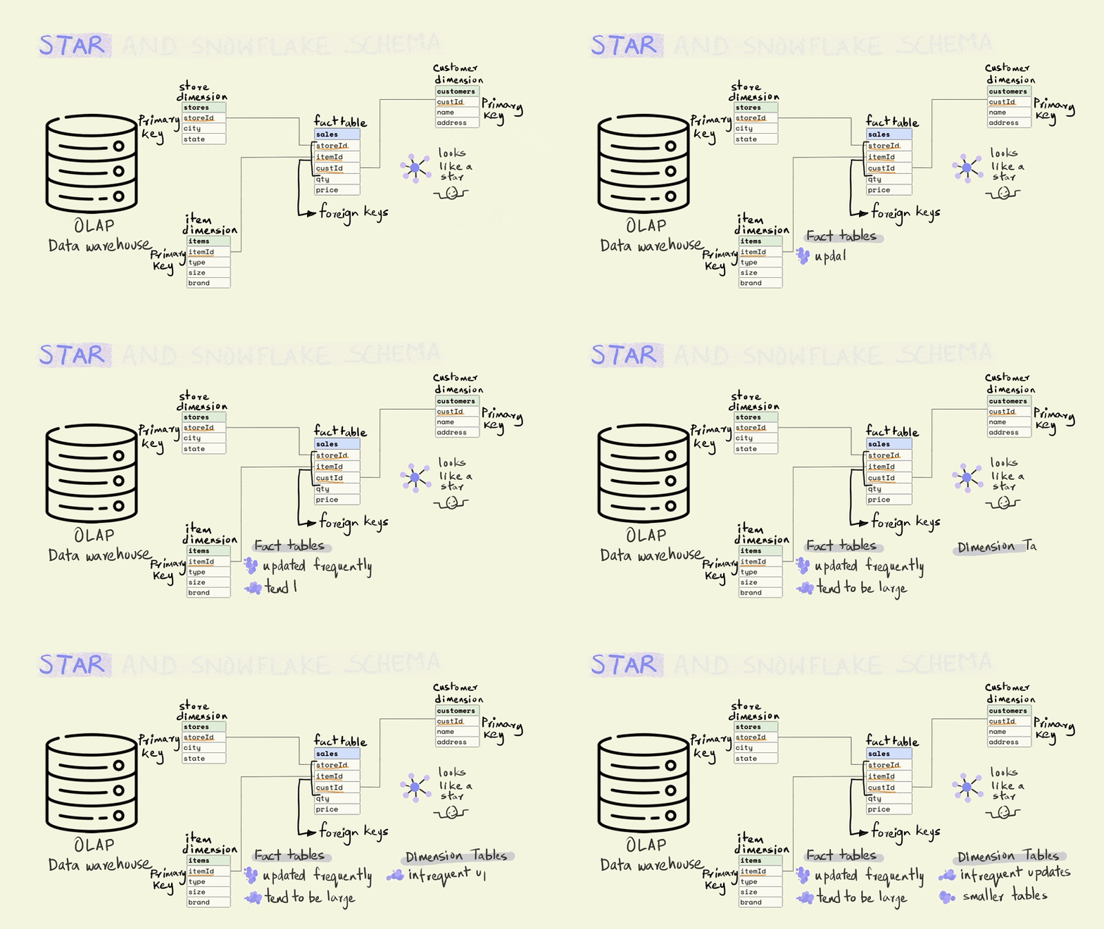
A star schema is the simplest and most widely used schema for organizing data in a warehouse. It has a central fact table that is surrounded by dimension tables. 

The fact table contains data on key business processes like sales, bank transactions, inventory, etc. For instance, in the illustration below, the fact being captured is the price and quantity of an item that was sold from a particular store to a particular customer (this would typically include a time component as well).

Stores, items, and customers constitute the dimensions of this fact. The dimension tables capture additional information about these dimensions. For example, the item table might include information about the type of item, the size, and the brand, while the store table might include the city and state that a store is located in.

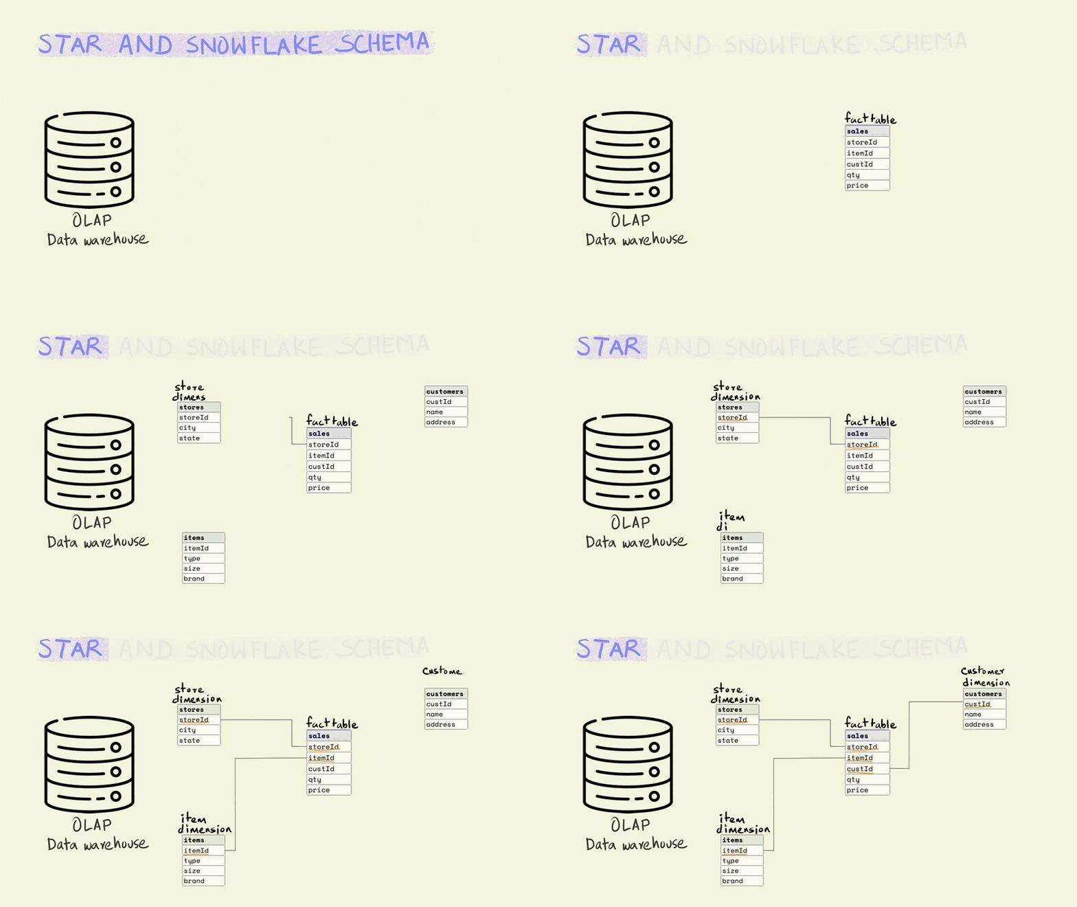
The different tables are linked to each other using keys. Keys are used to uniquely identify rows in a particular table. For instance, the storeId is the primary key for the store dimension and uniquely identifies the row that contains information about a particular store. The rows in a fact table are usually identified using a composite key that includes all the dimensions. In the illustration below, each row in the fact table is unique for the combination of store, item, and customer, i.e. there is only one row that shows the price and quantity of an item that was sold from a particular store to a particular customer.

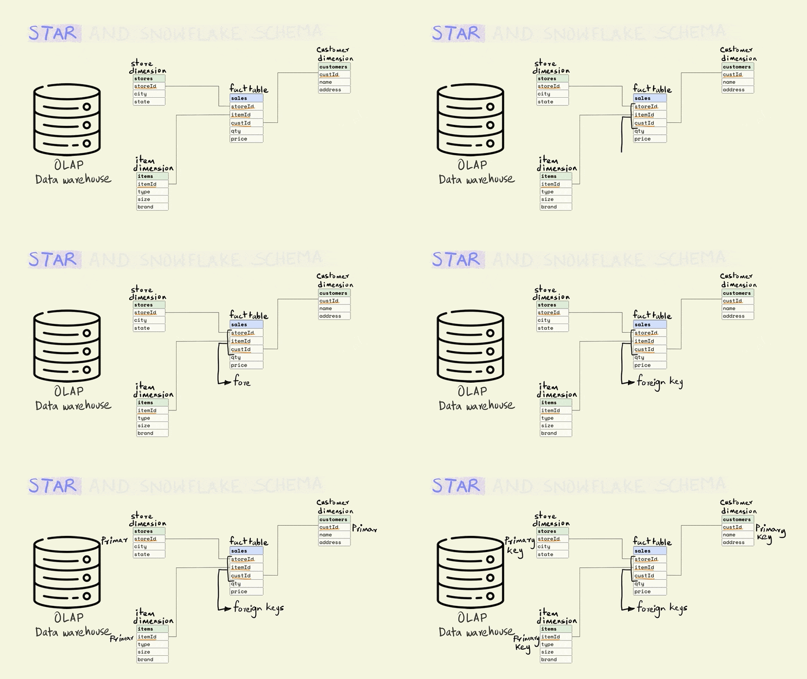
The name for the schema comes from the fact that it has a central fact table that is surrounded by dimension tables that make it look sort of like a star.

The fact table tends to be really large and is frequently updated. While the dimension tables are smaller and less frequently updated.

The snowflake schema is a more normalized version of the star schema. In the star schema there cannot be more than one level of dimensions, but the snowflake schema has no such restrictions.  

For instance, if we wanted to add additional information about the city that a store is located in, the star schema would require this to be added to the store dimension since it only allows a depth of one level for dimensions. This would mean that the data on a city could be duplicated if there were more than one store in a city. 

In the case of a snowflake schema, the information could be captured separately in a city dimension table as shown below.

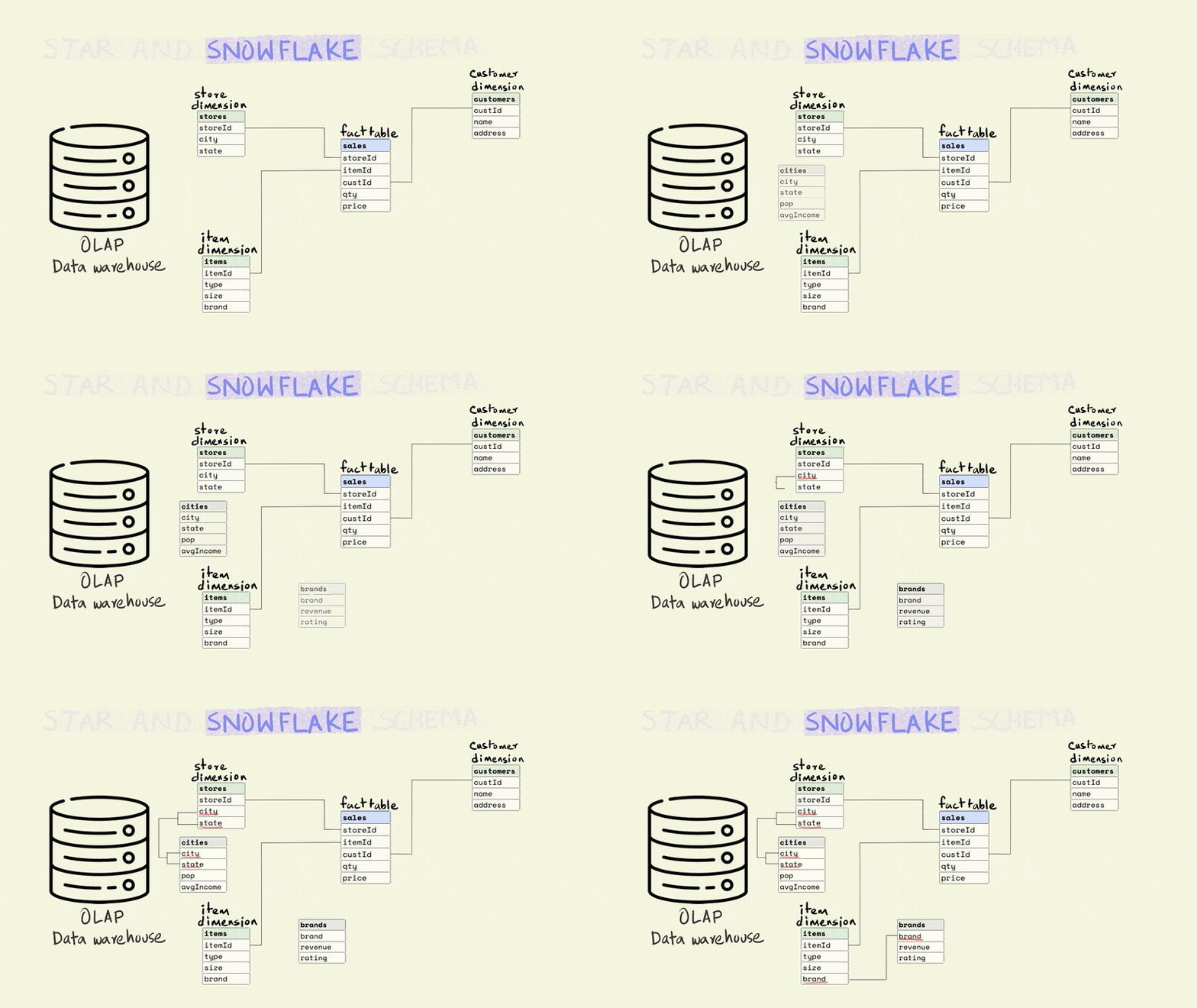
While the snowflake schema reduces data redundancy, it suffers from the same issues as stricter forms of normalization, since it requires joining more tables to perform analytical queries.

A sample query

Let’s round things off with a sample OLAP query. Most OLAP queries use the following set of operations:

1. Joins: To combine information from different tables using the common keys
2. Filter: Identify rows that match certain criteria
3. Aggregate: Calculate aggregate statistics across different groups in the data. For instance, find the average sales by region.

Let’s use an example to explore these common OLAP operations.

Assume that we want to understand how sales relate to the average income of the states they are located in using the tables shown in the illustration, but we only want to include stores that are located in cities with more than a million people.

The fact table only contains information for the daily sales for different stores. The stores dimension table contains the name of the city and state that a store is located in, while the city dimension includes the name of the city and state along with the population and average income.

The first task is to combine the store and cities tables. This would give us a table with each store, along with  information on the population and average income for the city in which it is located.

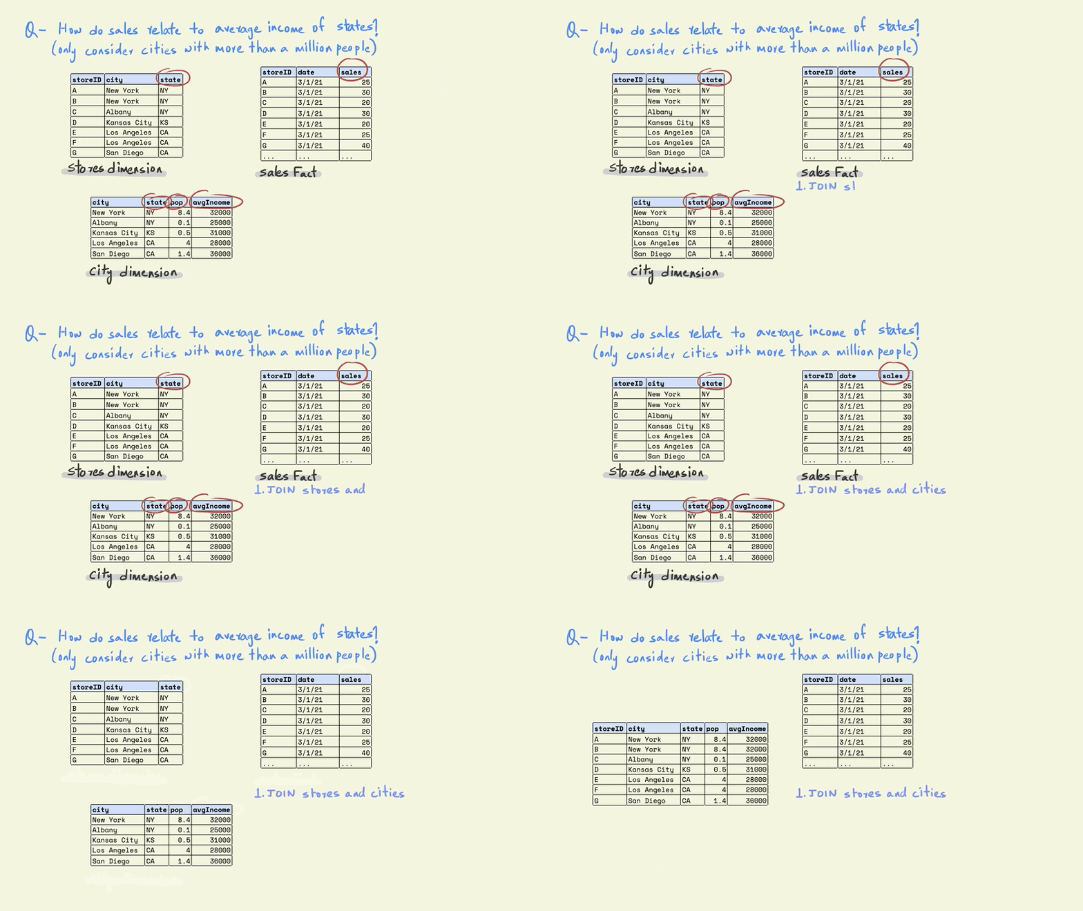
The next step is to filter the rows in the table so that we only keep those that are in cities with a population greater than one million.

Now this smaller table can be combined with the larger sales table.

Next, we can group this table on the states to calculate the average store sales and income for each state.

OLAP encompasses a lot more than we can cover here. If you would like to learn more, I highly recommend these free courses that are available through EdX here.  Moreover, we only touched on OLAP solutions that use the relational data model where tables are connected to each other using keys. There is an entire space of database analytics called NoSQL that uses more complicated non-tabular data models to store and analyze data. You can learn more about them here. Finally, Kinetica is one of the fastest databases in the world. It combines the ease of use of the traditional relational data models with cutting edge speed of vectorization to serve the OLAP needs of modern enterprises. Give us a try for free.

Hari Subhash is Sr. Manager of Technical Training and Enablement at Kinetica.