Time Series Analytics

There are useful timestamp functions in SQL, Python, and other languages.  But, time series analysis is quite different. Times series data is often never-ending measurements in a points-in-time sequence.  The data is almost painful to the human eye but fits well  into computers.  Time series analysis find correlations, conflicts, trends, or seasonal insights using sophisticated mathematics.  It reveals the factors that influence product quality, profit margins, pricing, machine failures, and other business results.

Time stamped data.

This is the domain of spreadsheets and traditional database layouts.  Sometimes, these relational tables use temporal SQL. But to be clear, temporal tables are not time-series data. 

Account ID	Customer	Transaction	Date	Time	ATM ID
9876543-01	Eric Rossum	$200.00	06/18/23	15:10.502726	Mybank98892-A14
9876543-01	Eric Rossum	$160.00	07/27/23	12:28.470988	Mybank98892-A10

Times series data  

An example of one array record is:

07/02/23,0.110000077,-0.2663,0.0408,0.9785,-0.0004,0.0058, 0.120000084,-0.2631,0.03749,0.973359,-0.0004,0.0058,0.130000127,-.24411.017982, 0.940882,-0.0028,0.0021, 

+200 more measurements.

Reformatted it might look like this table:

Date	time	gFx	gFy	gFz	wx	wy
07/02/23	0.110000077	-0.2663	0.04080	0.978500	-0.0004	0.0058
07/02/23	0.120000084	-0.2631	0.03749	0.973359	-0.0004	0.0058
07/02/23	0.130000127	-.24411	.017982	0.940882	-0.0028	0.0021

Time series data can fill entire memory banks with measurements and time-stamp separators. After the first few records, the human eye says “I’m leaving” –but the computer loves it!  Time-series data often arrives in 10s or 100s of terabytes.  Today, with cloud computing, anyone can grab 20 or 100 compute servers for 30 minutes.  The power to number-crunch 500 terabytes of data is at our fingertips. Big data indeed! 

Big data from the 2010s is small compared to what programmers are wrestling with in the 2020s. Volumes are up as are real-time use cases. Consider Boeing and Airbus. They collect petabytes of airplane sensor data annually. Every industry is analyzing bigger data.  According to G2 analysts[i] “In 2023, we will generate nearly 3 times the volume of data generated in 2019. By 2025, people will create more than 181 ZB of data. That’s 181, followed by 21 zeros.”  Data is arriving faster too.  Confluent’s State of Data in Motion Report found that “97% of companies around the world are using streaming data… More than half of this group (56%) reported revenue growth higher… than their competitors” [ii]

Time Series Analysis Use Cases

Time series analysis began long ago with stock markets and risk analysis. Today it is vital for the Internet of Things, fraud detection, and dozens of other workloads. While many of these use cases may sound familiar, the data and algorithms are far from it. 

Industry	Use Cases
Financial Services	Cyber threat hunting, ransomware detection and response, multi-channel risk correlation, valuation prediction, yield projections, securities trading sympathy alignments, finance supply-chains
Healthcare & Life Sciences	Remote patient glucose monitoring, air pollution tracking, chronic disease correlation, seasonal drug sales by illness, pharmacy drug sales versus outcomes, health wearables correlation
Insurance	Insure vehicles by the mile, fleet telematics pricing, consumption-based machines or premises contracts, seasonal risk analysis, home owners & auto policies future premium costs, forecast future value of a claim
Manufacturing	Precision agriculture, digital twins simulation, near real-time demand forecasts, variable speed supply-chain optimization, yield optimization, end-to-end root-cause analysis, products-as-a-service pricing & maintenance,
Oil & Gas	Digital twins simulation, exploration drilling and production, smart energy grid reliability, battery optimization, supply-chain risks, cyber threat hunting, wellbore positioning, predictive maintenance,
Public Sector	Smart cities traffic monitoring, disease track & trace control, events + crowd management, civic projects vis-a-vis property valuations, water and trash management, near real time cyber threat hunting
Retail	Real-time supply chain orchestration, supply chains cyber risk, precision seasonal inventory, item delivery disruption, inventory & warehouse optimization, recovery/reuse discarded shipping assets, cold case monitoring
Telecommunications	Seasonal & long-term network capacity surges, multivariate network traffic prediction by month, high data center transmission gridlock prediction, parts & work routes planning, 5G warehouse automated guided vehicles tracking
Travel & Transportation	Connected cars, last-mile multimodal transport options, fleet management, driver & passenger safety, dock schedule optimization, fuel economy optimization, predictive repairs, capacity optimization, seasonal fares optimization, derailment prevention, transportation-as-a-service pricing
Utilities	Electric vehicle charging planning, energy grid aggregate consumption, severe weather planning, transmission resilience, generation optimization, grid-modernization, real time grid faults/capacity surges, cyber threats

Wrestling with Complexity

Time series analysis involves sophisticated mathematics applied to huge arrays of data. Hence, there are dozens of time series algorithms from universities, GitHub, and vendors.  Kinetica was an early adopter of “bring your own algorithm” integration. Today its simple to run your favorite algorithms in parallel. Here are a few examples of bring-your-own-algorithms (BYOA):

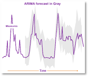
ARIMA: The Auto Regressive Integrated Moving Average can summarize trend lines. It then can predict highs and lows that might occur. Its flexible and outstanding at forecasting sales trends, manufacturing yields, or stock prices. This is a popular algorithm to get started. 

Shapelets are a category of algorithms that smooth out the sawtooth pattern measurements.  There are many times when a 0.03% value change is irrelevant – especially with sensor data.  Shapelets make it easier to compare and correlate data streams. 

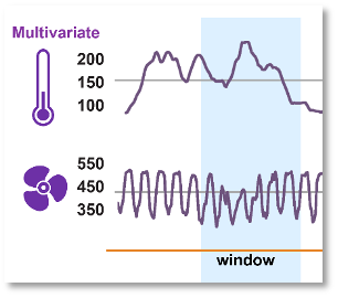
Multivariate time series classification algorithms detect correlations from different measurement scales. We can’t compare wind speed and propeller temperature numbers on a small airplane.  But we can see correlations between the graphs which the multivariate classification detects.

Vector similarity search is the latest breakthrough in time-series analysis.  Similarity-based searches do rapid pattern matching and data analysis.  This accelerates cyber-security, recommendation engines, image, and video searches. A key benefit is comparing time-series data points that have no relationships keys or name-identifiers.  Matches can be similar instead of identical data.  Vector similarity search enables proactive monitoring, predictive maintenance, and real-time anomaly detection.

Kinetica’s Best Fit with Time-Series Analysis

Kinetica is a time-series database with several capabilities that accelerate time-series analytics. These are:

Window functions: Built-in sliding windows help correlate events that occur in close time-proximity.   It’s easy to set the start and width of the window. Within the window, numerous algorithms can find important events or results.  For example, moving averages can detect which four or more events are causing price surges or machine failures. The time-period can be minutes, weeks, even months. We can then compare the sliding average to different points throughout the year.

Data loading: Kinetica set out to speed-load data was a necessity for their first few customers. Some of them required Kafka data streams loaded and analyzed within 10 seconds. This was foundational to Kinetica’s earliest product development.  Kinetica has three features for faster data loading:

• Kinetica database ingests direct into the cluster.  Data doesn’t pass through a central point of control. This scales better, has no single point of failure, and new nodes can be added without disruption.
• Kinetica’s native Kafka integration accesses Kafka topics using Kafka Connect.  Once a stream begins, there are minimal latencies for Kafka writing streams to disk. 
•  Kinetica’s lockless architecture avoids the heavy overhead of conflict resolution in many database engines.  We use versioning and optimistic concurrency control to ensure consistency and isolation. This enables faster processing and less contention for resources in analytical workloads. 

High Cardinality Joins: Time-series data often involves joining dozens of data streams with unique values together.  Multi-server parallel clusters are essential to handle big data high cardinality joins. What is high cardinality? Cardinality is high when a table column has thousands or millions of unique values. A table column containing only “Yes” or “no” has a cardinality of two. The receipt total for the 37 million who shop at Walmart every day is near 37M cardinality.   Joining two tables on high cardinality columns is computationally intensive.  It’s often an intolerable meltdown. Every value in the first table must be compared to every value in the other table for a match.  Imagine table-A has 100,000 unique values and Table B has 50,000,000 unique values. The computer must then match 100,000 * 50,000,000 memory cells –a mere five trillion comparisons.[iii] 

Why are high cardinality joins common in time-series data?  Start with time itself which is often stored in hours-minutes-seconds-and-milliseconds.  There is enough drift in clock ticks to make most every time value unique for months.  Other data with wildly unique values includes temperatures, identification numbers, stock prices, airflow, ocean currents, traffic patterns, and heart monitors.  Bigdata joins are inescapable.  Kinetica’s super-power comes to the rescue.   

GPUs and Intel AVX performance boosts: Vector processing in GPUs or Intel CPUs is perfectly suited for high cardinality joins.  Kinetica leverages hardware vectorization in GPU devices or Intel AVX instructions.  Start up a few cloud instances of NVidia A10s to exploit 9,200 optimized CUDA cores. It’s a clear competitive advantage for you and Kinetica. You might have time to run down the hall for a coffee refill. Performance of this intensity accelerates your productivity.  It also enables jobs to be rerun to improve analytic accuracy.

Kinetica finishes complex joins long before programming languages and other software tools.  You will want Kinetica software to do that for you. A table join of 20 terabytes to 50 terabytes doesn’t have to mean waiting hours for results.  The alternative is slow performance and many days of manual work-arounds.

Running Your Code in Parallel: Another foundational experience taught Kinetica engineers that customers wanted to use any algorithms. The data scientists had compelling reasons. Kinetica developers made it easy to bring-your-own-algorithm.  Your algorithms becomes a User Defined Function (UDF).  Kinetica software runs your UDF code in parallel, a benefit not found in many DBMS.  There are UDFs available on Github for data cleansing, data transformations, parsing, aggregations, and –best of all– data science.  There are many good UDF tutorials on Kinetica web pages.  Most developers can integrate their favorite algorithms easily.  Many years of Kinetica enhancements are accessible here.

Bonus:  The human eye is a powerful analytic tool.  People see graphical data patterns in an instant.  So Kinetica renders gigabytes of graphical data fast and condensed.  We then send it to visualization tools like Tableau or PowerBI.  That means Kinetica won’t overload the business intelligence servers or the network.  The user can quickly spot anomalies and start drilling into the discovery. 

Summary

Kinetica fits well into time-series data preparation and analysis. It helps with understanding the dataset and its context.  It accelerates data exploration, data munging, analytics, and feature engineering.  Each of these tasks requires multiple processing steps. These tasks involve detailed work and are often time consuming. Time-series data also drives the data analyst to make a lot of complex decisions.  This includes selecting the right tools and methods. When Kinetica provides these functions, the entire data preparation is done in situ.  There’s much less data movement –a time consuming low value task.  Furthermore, Kinetica functions enable preparation of big data time-series analysis. Bring your own algorithms!  Kinetica speeds all these things up. Including you.

---

[i] https://www.g2.com/articles/big-data-statistics
[ii] https://www.confluent.io/data-in-motion-report/
[iii] https://archive.kinetica.com/blog/dealing-with-extreme-cardinality-joins/